Hi all,
Happy new year! I’m applying ogs5py on python to simulate a coupled system which includes both heat transport and groundwater flow. Due to the required precision, my mesh file was generated by over 30000 points. In my time block, there are 73 time-steps. However, it took more than 3 hours to simulate this model. In addition, there is a constant groundwater flow in both x and y directions. I’ve tried to consider an initial head setting for all points but it doesn’t work. Besides, I have considered a doublet in my model. The result shows that there are some points where their temperatures are below the lowest setting temperature and some points which have a relative higher temperature than the given highest setting temperature. Although the difference is small, it looks weird. simulation2_root.zip (26.0 MB)
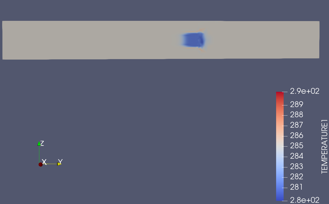
For example, in this result(10th time step), the background temperature is 285 K. Before this moment, there is water injected into the well and the temperature of the water is 281 K. Besides, a part of water would be pumped out from another well which couldn’t be seen from this figure. But it doesn’t matter as the pumping would not influence the temperature.
However, when I zoom in, I find that there are some places where the temperature is higher than 285 K which is extremely strange. And also the temperature is lower than 281 K at some points.

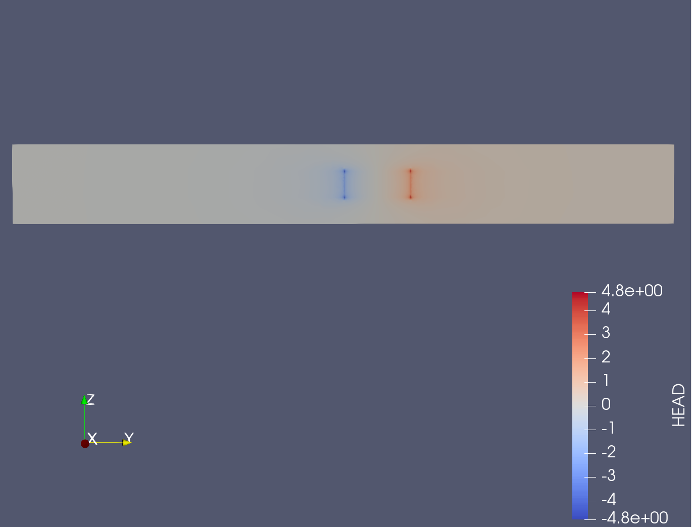
Besides, according to the head distribution figure, there is also something wrong happening. In my source term block, the water would be either pumped out or injected in two wells. In theory, the head should be same along the polyline where the screen of wells is located. However, from the figure, the head seems to be higher or lower at the top and bottom two points.
I guess, this is because your DIS-TYPE is CONSTANT, please try CONSTANT_NEUMANN
The simulation should not take that long, but it could be. However, it seem that you are having some oscillations.
I will have to look at it more detailed.
Hi Thomas,
Thanks, it works well. But the result shows a big difference between the thresholds of head. I guess it’s because the units of the CONSTANT and CONSTANT_NEUMANN are different. In my model, the water would be pumping from or injecting to wells in given flow (m3/s). And in CONSTANT_NEUMANN documentation, it is said that * CONSTANT_NEUMANN double (assigns the value multiplied by node area/node length to each node. Is there any method that I can transfer the flow into suitable unit for CONSTANT_NEUMANN?
Please try following in your NUM file:
GeoSys-NUM: Numerical Parameter ----------------------------------------
#NUMERICS
$PCS_TYPE
GROUNDWATER_FLOW
$LINEAR_SOLVER
; method error_tolerance max_iterations theta precond storage
2 5 1.e-06 1000 1.0 1 2
#NUMERICS
$PCS_TYPE
HEAT_TRANSPORT
$LINEAR_SOLVER
; method error_tolerance max_iterations theta precond storage
2 5 1.e-010 1000 1.0 1 2
#STOP
With that: my Laptop solve your model in 860 seconds
Note: For the output I use Paraview with PVD for the whole Domain and each timestep:
#OUTPUT
$PCS_TYPE
GROUNDWATER_FLOW
$NOD_VALUES
HEAD
$GEO_TYPE
DOMAIN
$TIM_TYPE
STEPS 1
$DAT_TYPE
PVD
#OUTPUT
$PCS_TYPE
HEAT_TRANSPORT
$NOD_VALUES
TEMPERATURE1
$GEO_TYPE
DOMAIN
$TIM_TYPE
STEPS 1
$DAT_TYPE
PVD
#STOP
For each process, please add
$BOUNDARY_CONDITION_OUTPUT to your PCS File.
You will find 2 new files: simulation2_GROUNDWATER_FLOW_BC_ST.asc and simulation2_HEAT_TRANSPORT_BC_ST.asc
These files shows the node index and the real assigned values of ST and BC per node.
There you can see that you inject 9 x 1 m3/s per polyline. Your polyline is having a length of 40m, according to you GLI file. Therefore 9/40 =0.225 and
CONSTANT_NEUMANN 0.225
In the ASC file you will find your node-wise assignment changed in:
5.625E-01
1.125E+00
1.125E+00
1.125E+00
1.125E+00
1.125E+00
1.125E+00
1.125E+00
5.625E-01
Hi Thomas,
I tried the NUM file given by you. However, after several time step, there is a information: Warning in CRFProcess::ExecuteLinearSolver() - Maximum iteration number reached
Moreover, after 59 time steps, it shows ‘Diagonal near zero! Disable diagonal preconditioner!’. Then my model stops. And I wanna know when I should use NON_LINEAR_SOLVER and COUPLING_CONTRIL in NUM file. (In my model, the density of water would change with temperature.)
Well I solved it on a Win10 System. If you are using Linux then your NUM settings could be a bit different.
NON_LINEAR_SOLVER is used for non-linear processes, so for Groundwater you don’t need it.
Which process answers with: CRFProcess::ExecuteLinearSolver() - Maximum iteration number reached???
In HEAT TRANSPORT PROCESS. I’m using OS system now. Oh, I forgot to change the constant value in CONSTANT_NEUMANN. Now I’m running it again. Will see if it works fine.

Dear Hoyue_Liu. Very nice model! I think this is very helpful to the community. Thanks for posting the original data.
There are still some small oscillation in the results, coming from solving the first time step, I guess.
Hi,
Recently I’m trying to calculate the energy balance in my model. Now I’m doing with a simple model which includes only one well. Basic parameters: injecting water for 200 days: 1000 cubic meters per day with a temperature of 16 Celsius degree. The background temperature is 12 Celsius degree.
Thus, the energy injecting into my model should be Q = cm(16 - 12) = 4183 * 1000 * 1000 * 200 * 4 = 3.3464 * 10^12 J. However, according to my modelling result, the energy increased in my model is Qm = effective(cm) * sum(T - 12) = 7.15 * 10^15 J which is much more than the injected energy. I wonder if I used the right formula to calculate this.
Besides, there are many ways to do the advection calculation such as FD, MOC, VTD etc… I couldn’t find information about which method is applied in OGS5.
Hi Thomas,
Is there any way to get rid of the small oscillations from solving the first time step? I’ve tried to use smaller time step but does not work.
Best,
Haoyue
Difficult I think. You can refine the mesh along the injection well and then reduce the timestep size.
You can also try to only increase the timestep size with the same mesh so you maybe don’t see that effect, but I’m not sure if that works in your case.
Or you give a different initial condition (file based) at the beginning, which already contains a gradient around the wells