Map NetCDF data on OGS surface meshes
This tutorials will show you some examples how to map data from NetCDF file format to OGS surface meshes.
Mapping NetCDF data on ogs_mesh.vtu can be necessary when you want to use Satellite data or data from other simulation software such as mHM as input data that uses the NetCDF format.
The first example will show you how to map output data from mHM as point data on an OGS mesh.
Example 1: Map mHM output data as point data on OGS mesh
In this example, we will map mHM output data containing soil water content (scw) of Germany onto an ogs_mesh.vtu of a part of the Selke river catchment using ParaView (tutorial_swc.pvsm).
Therefore the NetCDF formatted data has to be imported in ParaView, its coordinate system has to be transformed to the coordinate system of the ogs_mesh.vtu, then the data has to be mapped (Figure 1).
The corresponding files including a state file for ParaView can be downloaded here, PW: tutorial_swc.

Import NetCDF file:
Let’s get started. At first read in the NetCDF file. Usually NetCDF is a raster based–file format.
This means that a raster (unifrom grid) is defined as an array. Each raster/array cell is defined by coordinates of the cell center and variables (e.g. soil water content) linked to the raster cell.
For time-dependent data, usually one array per time step is defined.
Click File->Open select swc.nc. A prompt will asks you to specify a NetCDF reader as there are different NetCDF formats out there. As swc.nc uses the CF conventions, choose NetCDF Reader. swc.nc will show up in the pipeline browser. mHM NetCDF files do have unregular cell coordinates, which is not ideal for ParaView to import. We need a little trick.
Just uncheck Spherical coordinates to read in the coordinates as cartesian; click Apply. Sometimes it may be necessary to first check Spherical coordinates, click apply, then uncheck Spherical coordinatesand click Apply again.
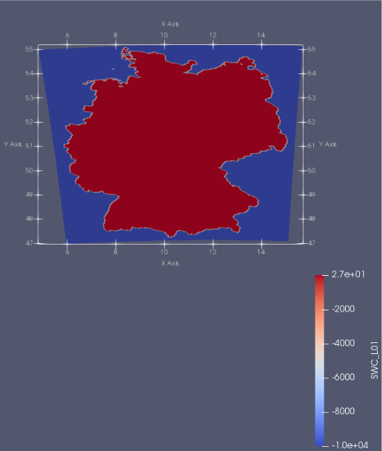
Your imported data should look like in Figure 2, containing longitude and latitude as coordinates.
It’s output type should be vtkStructuredGrid' . Unfortunately, the cell centered points of the original NetCDF file are now vertices of quadriliteral cells in the vtkStructuredGrid`. The cells are now shifted in x and y direction, so we need another trick later on. Before we need to transfrom the longitude–latitude coordinates.
Transform the coordinate system:
Afterwards, you have to transform the coordiante system from longitude–latitude (EPSG:4326) to Gauss–Kruger (EPSG:5684), which is used by this ogs_mesh.vtu. Gauss–Kruger–4 is a cartesisn coordinate system that uses m as units. Therfore we will use a ProgrammableFilter to include a python script. Within the python script we use the library pyproj for the cordinate transformation. You have to install it into your local python folder as there is no option to install in the python version that comes with ParaView—let’s say it did not find any. In case you have a C compiler installed you can install pyproj using pip via pip install pyproj. Make shure that you have the same python version as used by ParaView. If you do not have any C compiler installed, which can be the case on Windows, then download the corresponding precompiled python wheel file (cpXX in the filename reflects the python version) and install via pip install pyproj‑2.2.2‑cp38‑cp38‑win_amd64.whl (example). After installing pyproj you gotta tell ParaView were this library is located. Just open a python shell in ParaView and add the directory were you installed pyproj to the system path:
sys.path.append('path/to/pyproj')
Ok. No right–click on swc.nc in the pipeline browser and then Add Filter -> Alphabetical -> ProgrammableFilter.
In the added filter set Output Data Set Type to Same as Input add the following script:
from pyproj import Transformer, transform
import numpy as np

# read in data
input = inputs[0]
longitude = input.Points[:,0]
latitude = input.Points[:,1]

# define coordinate transform function by defining the coordinates
# systems of input and desired output
transf = Transformer.from_crs(
                    "EPSG:4326",
                    "EPSG:5684",
                    always_xy=True)

# define x and y as np-arrays
x = np.empty(len(longitude), dtype=np.float64)
y = np.empty(len(longitude), dtype=np.float64)

for i in xrange(0, len(longitude)):
    dest = transf.transform(longitude[i],
                     latitude[i])
    x[i] = dest[0]
    y[i] = dest[1]

# write output
output.Points[:,0] = x
output.Points[:,1] = y
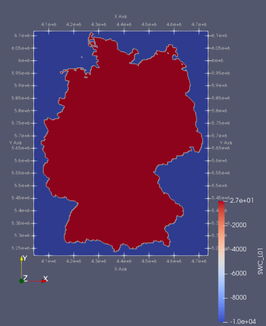
Important: In python3, the function xrange was renamed to range. The output should look as in Figure 3.
Extract grid points: To solve the problem with the shifted cells, we now take the ProgrammableFilter, extract all points out of it and add new cells based on the extracted points. Just right-click on ProgrammableFilter in the pipeline browser, then Add Filter->ExtractSelection. Now select all points on the grid by using the Select Points on (d) function in the upper panel of the render view and click Copy Active Selection in the Properties Panel. Then hit Apply. The output is an vtkUnstructuredGrid that conists of the same number of points and vertex cells (zero–dimensional cell); there should not be any edges. Okay, now we are ready to import the OGS mesh.
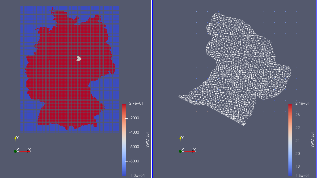
Import ogs_mesh.vtu: Now you can read in the ogs_mesh.vtu via File->Open. When viewing the the ogs_mesh.vtu and the output of ExtractSelection together, you can see that the OGS mesh is much smaller (Figure 4).
Reduce size of grid to ogs_mesh.vtu: To save some computation time we will cut out a mesh region that roughly fits the ogs_mesh.vtu file geometry using the filter Clip. Just right-click on ExtractSelection in the pipeline browser, then Add Filter->Alphabetical->Clip. Set Click Typeto Plane; the Origin close to the right side boundary of the ogs_mesh.vtu and Normal to 1; 0; 0.
Click Apply. It wil cut out everything right of the clipping plane. Just repeat this to cut out the remaining sides; hit Invert when clipping the left and the down side. The output is shown in Figure 4.
Map data onto ogs_mesh.vtu:
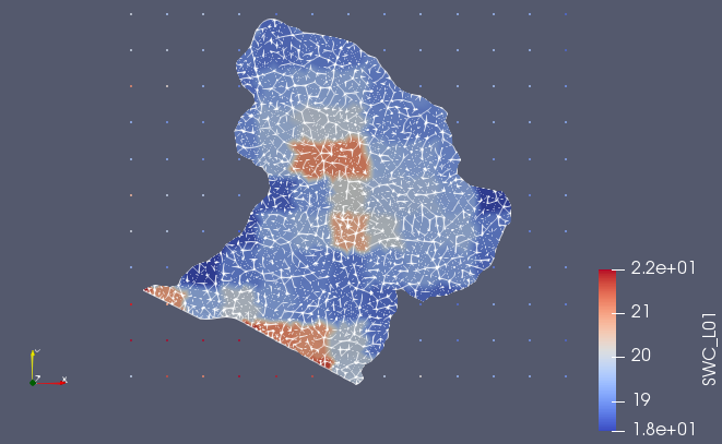
a) Finally we can now map the data of the volume on the ogs_mesh.vtu by adding a PointDatasetInterpolator filter. Set Input to the prior filter (either the Clip or the ExtractSelection) and Source to the ogs_mesh.vtu. Use the VoronoiKernel as Kernel (interpolation algorighm) and set Null Value to -9999. The VoronoiKernel uses the value of the closest point in the Input grid as interpolation value for a point in the Source grid. Tutorials on other interpolation algorithm will follow.
The output mesh is a vtkUnstructuredGrid of ogs_mesh.vtu with the point data of SWC_L01, SWC_L02 (Figure 5). Note that the mapping also finishes if the both grids do not overlap completely!
b) The new grid does only contain the interpolated point data. To retrieve the original cell and field data of ogs_mesh.vtu we need to combine both data sets by using the AppendAttributes filter. Just highlight the original imported ogs_mesh.vtu and the PointDatasetInterpolator filter and right click, Add Filter->AppendAttributes. This should output an vtkUnstructuredGrid that contains the interpolated point data and all data of the original ogs_mesh.vtu.
Save Output:
To save the file highlight AppendAttributesand click File->Save Data. By choosing PVD as file format you can export a file series of VTU’s (one VTU per time step) that are linked within a PVD file. By choosing VTU you have the choice to ouput either as file seriess (one VTU per time step) but without a linking PVD or to gather the data of all time steps in one file. The latter option did not work for (ParaView 5.6.2, Ubuntu 18.04 LTS).
Please comment if there are problems or if something is not clear.