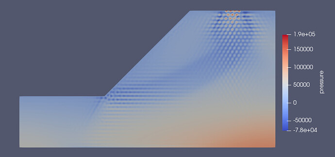
Dear OGS Team and Prof. @Thomas_Nagel
I am solving a coupled HM problem (up formulation) for slope stability analysis under fully saturated conditions with a load at the top of the slope crest. However, I am getting spurious oscillations in the pressure wave during my simulations (Figure attached). I learned that it is the typical incompressibility constraint for hydromechanically coupled problems as I do not meet the Ladyzhenskaya-Babuška- Brezzi (LBB) stability condition.
I found several ways to overcome this problem by using various stabilization methods (e.g., White and Borja, 2008). But the easiest way to eliminate the instability is by choosing a Q9P4 element (i.e., 9 nodded quad for displacement/4 noded quad for pressure).
I would like to know if there is any way of using the Q9P4 element in OGS for the HM problem. Also, I am open to knowing other possibilities for solving this numerical issue.
Thanks
Pavan.
Hi Pavan. You’re right. Nice example of the instability, actually. We typically use Serendipity elements in OGS (Q8P4) for this. You have to convert your mesh to quadratic elements (there’s a tool in your bin folder for that, just ls for Quadratic). Don’t forget to also convert the boundary meshes along with that.
Then, you set the integration order to 3 in your input file and the order of the displacements in process variables to two, leaving pressure at one.
Th
PS: simple example is here: Tests/Data/HydroMechanics/Linear/Confined_Compression/square_1e2.prj · master · ogs / ogs · GitLab
Thank you very much for the prompt response, Prof. @Thomas_Nagel
It worked. The interpolated pressure seems continuous. However, the pressure (i.e., primary variable) still has the shocks. Similar observations were seen in the suggested example by you. As far as the representation of pressure contours is concerned, the interpolated pressures will do the job.
However, I think the oscillating pressure values still affect the mechanics through its coupling term because the mechanics’ module is coupled by the pressure but not with the interpolated pressure.
Also, I observed more significant oscillations in pressure while using Q8P4 elements than T3 elements. Moreover, the interpolated pressures are continuous for Q8P4 elements.
Any thoughts on this?
Pavan.
This is just a plotting artefact, as pressure does not formally exist in the edge-center nodes. So You have to plot interpolated pressure. If that’s fine, then your solution is fine.
1 Like
Now I get it. Thanks, Prof. Nagel.
Dear Prof. @Thomas_Nagel
Thank you for your help and support earlier.
Inline with the same problem, I have a question. I am having difficulty deciding the success of the initialisation step for slope stability analysis under saturated conditions. To start with, I have considered the HM process in the same slope stability problem given in the benchmark examples (Link)
I have tried three different ways of initialising pore pressures and initial stresses.
- Using the incremental time stepping for activating gravity as indicated in the example until 1-second pseudo timestep (Link)
- Defining the pore pressures and initial stresses using the functional parameters following the ground equilibrium benchmark example (Link)
- Employing the second approach by using a Python code and assigning the pressures and initial effective stress using
MeshNode and MeshElement type parameters to the mesh file before starting the simulations. Then, using the following line for equilibration.
<compensate_non_equilibrium_initial_residuum>true</compensate_non_equilibrium_initial_residuum>
However, the problem is as the ground surface is not flat but sloped, I find it hard to decide whether I have successfully initialised pore pressures and initial stresses before applying any external loads. All the above-mentioned approaches result in dissimilar pressure and initial stress distributions.
Could you please tell me how to decide if the pressure and stresses are equilibrated and obtained correctly for a sloped geometry?
Thanks
Pavan.
Hi Pavan,
the stress field in the slope is probably not easily prescribed by equations, for the reasons you mention. Therefore, I’d stic with your first approach. However, you have to give the system time to relax to steady state, if it is HM coupled. In other words, excess PWP has to dissipate, consolidation finish. Then you have a valid initial state, from which you can restart whatever analysis you want to do.
Th
1 Like
Dear Prof. @Thomas_Nagel
Thank you for your help and support earlier.
I am writing to seek your assistance regarding the verification of the MohrCoulombAbboSloan model using the MTest code. Specifically, I am attempting to compare the peak stresses from the model with those predicted by the analytical Mohr-Coulomb (MC) equation.
For instance, with a friction angle (ϕ) of 33 degrees and cohesion (c) of 0, the peak major principal stress (σ1_peak) should theoretically match the MC equation:
σ1_peak = σ3*(tan(45+ϕ/2))^2
However, the peak deviatoric stress (q_peak = σ1_peak − σ3) obtained from MTest does not align with the analytical solution. I am curious whether this discrepancy could be attributed to the implementation of the MC model in MFront or if it might be related to the transition angle within the model.
My objective is to understand the differences between the Modified Cam-Clay (MCC) framework and the Mohr-Coulomb (MC) framework, particularly for applications in slope stability analysis. Hence, I am verifying and validating the stress-strain response as a preliminary investigation.
I have attached the relevant Python code for your perusal. Kindly help me in this regard.
Thanks
Pavan
MC_MTest.zip (277.5 KB)
